Inside Algolia Engine 4 — Textual search relevance

Julien Lemoine in Under the hood on Jul 7, 2016

We've changed how we search a lot over the last decade. For example, we used to begin every search by pressing Enter. Now it's no longer necessary - results appear as you type.

What people search has also changed.

Today’s search engines query much more than web sites and documents — they also query specific items like people, places, and products.

The Algolia engine was designed with these trends in mind. Algolia’s sweet spot is providing instant, relevant access to millions of small, structured records (and now from anywhere in the world). In this blog post, we’ll talk about how the Algolia engine computes textual relevance and why it works well for exactly these kinds of records. By textual relevance, we mean the letter and word-based aspect of ranking query results. Textual relevance does not include business relevance, which is used to provide a custom ranking based on non-textual information like price, number of followers or number of sales.

In a previous post we discussed how our ranking formula works, specifically how it uses a tie-breaking algorithm to rank each component of textual relevance one-by-one. In this post, we’ll look at each of the five individual components it uses in detail: number of typos, number of words, proximity of words, importance of attributes and exactness.

1. The five components of textual relevance

Each of these components address a unique relevance challenge while also playing their part in the global relevance calculation.

1.1 Number of typos

The number of typos criterion is the number of typos in the query when compared with text in the record. This criterion allows you to rank results containing typos below results with the correct spelling. For example, in a search for "Geox CEO", you would prefer to have the "Geox" result (a typo-free match) displayed before "Gox" (a 1-letter-off typo). This example has a twist—”Gox” is not actually a typo in the usual sense (it’s a correctly spelled proper noun) but it’s still possible that a user could have mistyped “Geox” when searching for it.


1st record:
Title: "**Geox** SpA: **CEO** and Executive"


2nd record:
Title: **"**Mt. **Gox** **CEO** Resigns From Bitcoin Foundation**"**

1.2 Number of words

The number of words criterion is the number of query words found in the record. This criterion applies when the query is performed with all words optional (a.k.a. an "OR query"), a technique commonly used to avoid displaying no results. Here’s a simple example. If you search for "supreme court apple" you would prefer to have the first record before the second one as it contains all 3 of the words in the query.


1st record:
Title: "**Supreme Court** turns away **Apple** appeal in e-books antitrust case"


2nd record:
Title: "**Supreme Court** upholds Obama’s health-law subsidies"

1.3 Proximity of words

The proximity of words criterion is the distance between the matched words in the result. It’s used to rank records where the query words are close to each other before records where the words are farther apart. In the example below, you can see two different results for the query "Michael Jackson". In the first record, the proximity criterion is 1 - the terms ‘Michael’ and ‘Jackson’ are right next to each other. In the second record, the proximity criterion is 7 because there are 6 words between the matching terms. A lower value is better, i.e. records with a lower proximity value will be ranked about records with a higher value.


1st record:
Title: "**Michael Jackson** songs radiate through Spike Lee's neighborhood celebration saluting the King of Pop"


2nd record:
Title: "**Michael** K. Williams found inspiration in Janet **Jackson**"

1.4 Importance of attributes

The importance of attributes criterion identifies the most important matching attribute(s) of the record. Since records can contain more than one attribute, it’s not uncommon for one query to match multiple attributes of the same record or different attributes of different records. However, a match of one attribute might be more important than another when it comes to ranking, and that’s precisely why we have the attribute criterion. An example is shown below. Given a query for “Netflix” in a collection of articles, you’d want the title attribute match to carry more weight than the description attribute, hence the title-matching record is displayed first.


1st record:
Title: "**Netflix** is making movies shunned by studios"

Description: "As the company moves into feature films with the release of “Beasts of No Nation” on its streaming service and simultaneously in a small number of theaters, it is creating the type of movies that studios no longer make."


2nd record:
Title: "The new documentary ‘What Happened, Miss Simone?’ takes a look at the life and legacy of Nina Simone"

Description: "The new Netflix documentary ‘What Happened, Miss Simone?’ takes a look at the life and legacy of the talented Nina Simone."

1.5 Exactness

The exactness criterion is the number of words that are matched exactly. This criterion is very important for building quality instant (search-as-you-type) experiences because it’s important to display full-word matches before prefix matches. See the example below. If you search for "Prince", you want the exact word match to appear before the match where “Prince” is being considered as a prefix of “Princess”.


1st record:
Title: "Reflections on **Prince**: My classmate, the rock star"


2nd record:
Title: "Spain’s **Prince**ss Cristina goes on trial"

2. How the criteria are computed

We’ve just seen what each criterion does and how it can be used to influence the ranking of search results. Next, let’s look at how the five criteria are computed and what we’ve done to make their computation efficient.

2.1 Computing the number of typos

In our previous post about Query Processing, we explained how alternative terms are added to queries. For each alternative term, we also have an associated number of typo criteria (which corresponds to the edit-distance). This value of the overall typo ranking criterion is the sum of all typos used to find the match. For example, if the record is found via 2 words having 1 typo each, the typo criterion value will be 2.

It’s a very good practice to have this criterion at the top of the ranking formula. However, there is one exception: typosquatting. If you operate a service with a lot of user-generated content, you might already be familiar with this problem. Let’s take Twitter as an example. If you search for "BarakObama" on Twitter (note the typo), you would want the official @BarackObama account to appear before the typosquatting account @BarakObama. However, today it does not (as of June 2016). Typosquatting is a complex and difficult challenge.

One way that we recommend to handle typosquatting is to add an isPopular boolean attribute to the record of popular accounts and then to put it in the ranking formula before the typo criterion. On Twitter, isPopular could be set to true if the account is verified. This approach ensures that the official account with a typo will be displayed before any typosquatting accounts, no need to hide any results. For this approach to work well, the number of records with isPopular set to true should be a relatively small percentage of the dataset (less than 1%).

2.1.1 Typo tolerance tuning

The Algolia engine provides several different ways to tune typo tolerance for specific words and attributes:

minWordSizefor1Typo and minWordSizefor2Typos: Specify the minimum number of characters in a query word before it can be considered as a 1 or 2 typo match.
allowTyposOnNumericTokens: Specify if typo tolerance is active on numeric tokens (numbers) present in the query.
disableTypoToleranceOnWords: Specify a list of words for which typo tolerance will be disabled.
disableTypoToleranceOnAttributes: Specify a list of attributes for which typo tolerance will be disabled.
Alternative corrections: Specify a set of alternative corrections with the associated number of typos.
advancedSyntax: Add quotes around query words to disable typo tolerance on them.

2.2 Computing the number of words

Computing this criterion is relatively easy, it’s just the number of words from the query that are present in the record. Each word might be matched exactly or matched by any alternative form (a typo, a prefix, a synonym, etc.).

The position of the words criterion in the ranking is important and will impact results. For example, the query "iphone case catalist" with all terms as optional will have two different ways to match the record "Catalyst Waterproof Case for iPhone 6/6S Orange":

If words is before typo in the ranking formula: The ranking will be set to words=3 and typo=1 as matching more words is important to the ranking (even if Catalyst is found via a typo).
If typo is before words in the ranking formula: The ranking will be set to words=2 and typo=0 as less typos are more important to the ranking (in this case it’s better to not match the Catalyst term and therefore not introduce a typo).

2.2.1 The removeWordsIfNoResults parameter

Because of situations like this, we usually recommend against performing queries with all terms optional. Instead, we recommend using a specific query parameter that we’ve added to the API to help with these types of situations. The removeWordsIfNoResults parameter instructs the engine to first test the query with all terms as mandatory, then progressively retry it with more and more words as optional until there are results. This parameter gives us the best of both worlds (predictable behavior and always showing results) and also does not pollute faceting results. When all terms are optional there is a large increase in the number of matched records, as only one matching word is required to add the record to a facet. For example, in a query for “iphone black case”, any black item will be matched which will have a big impact on the quality of the faceting.

2.3 Computing the proximity of words

The proximity criterion’s value is the sum of the proximity of all pairs of words that are next to each other in the query. Computing the proximity of "iphone release date" is done like this: proximity("iphone", "release") + proximity("release", "date").

The engine stores word positions at indexing time in order to efficiently compute proximity at query time. We define the distance between two words A and B as the shortest distance between any A and B in the record (A and B may appear more than once). We increase the distance by 1 if the match with the shortest distance is not in the queried order.

The computed proximity between two words is capped at 8. If the words "apple" and "iphone" are separated by a distance of 10 or 100 words, the distance will still be 8. The goal is to avoid creating different proximity values for words that are not used in remotely the same context. In practice, 8 words is a sizeable distance between any 2 words, even when it’s mostly common words between them. Capping the maximum proximity has two other advantages:

It helps our tie-breaking algorithm. A maximum distance of 8 means that we don't know if a distance between words of 10 is better than 100, and usually we don’t want to (it’s just noise). Capping the proximity at a small number prevents introducing false positives into the relevance calculation. More importantly, it lets the other criteria in the ranking formula take over when proximity values are not meaningfully differentiated.
It enables a lot of optimizations on the storage and computation side, as we will see.

2.3.1 How word positions are stored

As we index a document, we assign an integer position to each occurrence of each word. For example the string "Fast and Furious" would be indexed as:

"Fast" at position 0
"and" at position 1
"Furious" at position 2

Additionally, we assign positions to some word prefixes as described in our blog post about indexing prefixes.

The position is also used to efficiently store associated information:

We use a single value to store the position of each word in the text and which attribute it came from. We keep the position of the first 1000 words inside each attribute and associate an number to each attribute (the first attribute will have positions 0-999, the second attribute will have positions 1000-1999, etc.)
For multi-valued string attributes, we need to ensure that the last word of a string isn't considered to be next to the first word of the next string. To do that, we increment the first position of each string by 8 each time we move from one string to another. For example if a record contains the following “Actors” attribute, we will store the word "Diesel" with a position of 1 and the word "Paul" with a position of 10 (+8 compared to the value in the same string). This will generate a proximity of 8 if you type "Diesel Paul", which is the highest value for proximity.


{
 "Actors": [
   "Vin Diesel",
   "Paul Walker"
 ]
}

2.3.2 Bonus challenge: multi-word alternatives

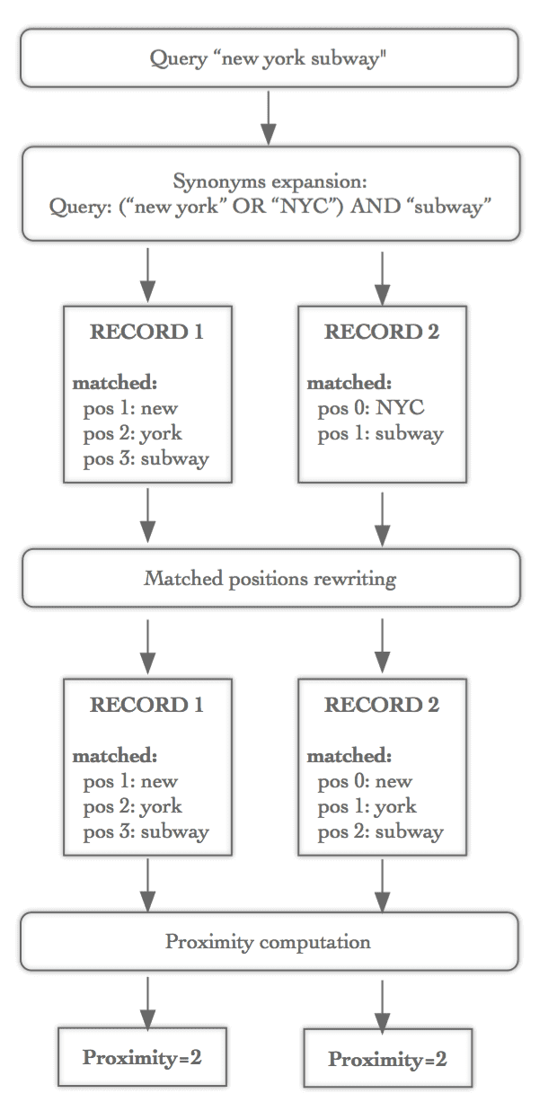
Computing a proximity distance can be very complex when you support alternative word matching, e.g. synonyms. If you have a synonym that defines "NYC" = "New York City" = "New York" = "NY", you would like to consider a record that contains "NYC" as strictly identical to a record that contains "New York". We solve this tricky problem by rewriting all word positions at query time.

Time for an example. Let's say that you have two different articles that you want to be searchable via a query for the "New York subway". You would like the proximity distance calculation to be the same between them. Here are the article titles:

"Why New York Subway Lines Are Missing Countdown Clocks"
"NYC subway math"

When this query is run, the first record will be matched via three words ("new" at position 1, "york" at position 2 and "subway" at position 3) and the second record will be matched via two words ("nyc" at position 0 and "subway" at position 1).

In order to avoid this inconsistency, we rewrite positions using a multi-word expansion. For the "NYC subway” query, we apply the following transformation:


- _"Nyc" at position 0 became:_
    - _Virtually "new"_ at position 0
    - Virtually "york" at position 1
- _"subway"_ _at position 1 became:_
    - "Subway" at position 2 because we introduced "york" word at position 1.

After the transformation, we have exactly the same proximity measure between the two records. This rewriting is entirely cumulative. For the "New York" query, if a record contains "NYC" at positions 5 and 15, it means that all original positions greater than 15 will be increased by 2 and all original positions between 6 and 15 will be increased by 1.

Example of position rewriting in multi-word synonyms

2.3.3 Attribute-aware proximity

When computing the proximity score, we don’t want to be misled when different parts of the search expression are found in different attributes of the record.

Say you’re looking for "soup of the day" and you have a record with "soup", "of the" and "the day" separately in three different attributes. In this case we do not want to compute a total distance of 10 (distance(soup, of)=8 + distance(of, the)=1 + distance(the, day)=1) because it would mean “of the day” are close together, which is not the case. Instead, we want a total distance of 17 (distance(soup, of)=8 + distance(of, the)=1 + distance(the, day)=8). The distance of 8 between "the" and "day" tells us that "day" was found in a different block than "of the". We use a dynamic programing algorithm to do this computation efficiently with a cost of O(N) (N being the number of matched positions).

2.3.4 Proximity computation tuning

The minProximity index setting allows to change the minimum proximity to something that fits your data better. If you set minProximity=2, it would mean that the query "New York City Subway" will have the same proximity score whether the record contains "New York City Subway" or "New York City's newest subway". The distance would normally be 1+1+1 for the first record and 1+1+2 for the second, but setting minProximity=2 means that all pairs of words with a distance less than or equal to minProximity are counted for 1. In this example, both records are given a proximity criterion score of 3.

2.4 Computing the most important attributes

As a reminder, the attribute criterion lets us say that a query match in some attributes is more important than others.

Each attribute is indexed as ordered or unordered (this is configured in the index settings). Indexing an attribute as ordered means that the position of the best matched word inside the attribute is taken into account during ranking. So earlier words will matter more. Indexing as unordered means that the position within the attribute is not taken into account. Word position is not important.

An example—if you index the title attribute as ordered and description attribute as unordered, the query “Netflix” will return the following 2 records in the order displayed.


1st record:
Title: “Cable fights **Netflix** to feed 'binge' TV viewers"
attribute=2: **Netflix** is the third word of the title attribute (title attribute is indexed with positions 0 to 999).


2nd record:
Title: "Deborah Ann Woll Previews ‘Daredevil’ Season Two",
Description: "Deborah Ann Woll, who co-stars as Karen Page on the **Netflix** superhero series “Daredevil”
attribute=1000: **Netflix** is found in the description attribute (the description attribute is indexed with positions 1000 to 1999 because it is the second indexed attribute). The attribute criterion is set to 1000 because the description attribute is indexed as unordered.

2.4.1 When proximity is before attribute in the ranking

There are two strategies to compute best-matched attributes and they depend on the relative position of proximity and attribute criteria in the ranking formula. Let's illustrate them by using the query "VMware CEO" to retrieve the following record:


Title: "**VMware's** chief drives three-pronged focus for virtualization software maker",
Description: "**VMware CEO** Patrick Gelsinger, in an interview, lays out the software maker's future in software-defined data centers, cloud computing and managing user devices like PCs and smartphones."

If proximity is before attribute in the ranking formula, we first find the location with the best proximity in the record and we then compute the best attribute on this location. On the record below, the query “VMware CEO” will have an attribute criterion of 1000 as the best proximity is found in the description attribute instead of the title attribute.
If attribute is before proximity, the best-matched attribute will be decided by the position of the best-matched word in the record. In this case, the query “VMware CEO” will have an attribute criterion of 0 as the best word is matched in the title attribute.

We recommend keeping the proximity criterion before attribute criterion. Proximity usually leads to a better identification of the best-matched attribute.

2.5 Computation of the exactness criterion

The exactness criterion represents the number of words that match entirely, not one as a prefix of another. This criterion works well when the query contains several words but the one-word case requires a modified approach. In an instant search use case, if a user has typed “was”, there is a greater chance that he or she might be in the middle of typing a search for “Washington” and not just stopping at the verb “was”. Displaying “was” before “Washington” in the results at that moment would not be ideal.

We have implemented three different ways to compute the exactness criterion for a single word query, each specified via the exactOnSingleWordQuery parameter:

exactOnSingleWordQuery=none: The exact criteria is set to 0 for all one-word queries.
exactOnSingleWordQuery=attribute: All records that have an attribute string exactly equal to the query will have exact=1. This option is the default as it works well for databases that contain names, brands, companies, etc.
exactOnSingleWordQuery=word: All records will have exact set to 1 if there is a word that matches exactly and is not in our stop word dictionary (see the removeStopWords option for more information). For the query “prince”, a record with “prince” will have exact=1 and a record with “princess” will have exact=0. For a query “was”, both records containing “was” and “Washington” will have exact=0 because “was” is in the stop word dictionary.

There is unfortunately no magic option that works well with all use cases, which is why we introduced the exactOnSingleWordQuery parameter. We recommend using exactOnSingleWordQuery=attribute if you have a database that contains lots of one-word entries like brand names, account names, movies, etc. We recommend using exactOnSingleWordQuery=word when you have content like titles that have a low probability of matching an entry using only one word.

2.6 Designed for small records

The five components of textual relevance we’ve discussed are uniquely designed for small, structured records. A few of them require some fairly complex processing, like the query-time rewriting of word positions for multi-word alternatives, but we think that having an approximation-free, exact value computation is worth it.

If you don’t automatically have small, structured records—i.e. if you’re starting with documents or long blocks of text—we recommended splitting them into multiple, shorter records. One record per paragraph is a good rule of thumb. This is the approach used by our DocSearch project, which crawls web pages containing technical documentation and can generate many records per page. DocSearch is now powering the search of 150+ open source projects, so there are lots of places you can try it out.

We’re constantly seeking more ways to customize relevance for advanced use cases. Some of the parameters presented in this post have been added to the API recently and several new parameters are currently being beta tested.

Not so long ago we were given a challenge: to index millions of articles of a popular news website and provide relevant results about the artist Prince’s death, even for queries with typos like "Prinse". The query “Prinse” matches article with "Prince" in the title (typo=1, words=1, proximity=0, attribute=0, exact=0) but the results were being displayed below other articles about "Sharon Prinsen" (typo=0, words=1, proximity=0, attribute=1000, exact=0) because it matches a prefix without typo. To solve this issue, we introduced a new option to consider all prefix matches as a typo: now all articles with “Prince” in the title will be served first (typo=1, words=1, proximity=0, attribute=0, exact=0) and articles mentioning "Sharon Prinsen" will come after (typo=1, words=1, proximity=0, attribut=1000, exact=0). With this improvement, we were able to address the relevance problem of prefixes while maintaining a high quality instant search experience.

Next readings

We hope this post gives you some insight into the inner workings of our engine and how we got where we are today. As always, we would love your feedback. Definitely leave us a comment if you have any questions or ideas for the next blog in the series.

I look forward to reading your thoughts and comments on this post and continuing to explain how our engine is implemented internally. Transparency is part of our DNA! :)

We recommend reading the other posts of this series:

tech blog.Developer's Rooftop

// words behind the code